The idea in one minuteA looped transformer reuses the same block of layers to refine a hidden state. More iterations buy more computation without adding model weights. The useful question is whether that extra computation improves the answer, and how to train it without storing every intermediate state.
Read the mechanics: the recurrence, one loop pass, a worked carry example.
Go deeper: training and gradients, adaptive stopping, the evidence, the criticism.
Why this, why now
For most of the scaling era, the levers were two: parameters and data. Then o1 and R1 made a third lever legible - test-time compute - and the entire reasoning-model boom has been one particular way of pulling it: generate more tokens. Chain-of-thought is, mechanically, a loop: the model writes a thought, reads it back, writes the next one. The state of the loop is the context window, the step size is one token, and the loop runs in vocabulary space.
There is another way to pull the same lever. Instead of looping over generated tokens, loop over depth: take a block of transformer layers, tie its weights, and run it again and again on the same hidden state. The state of this loop is the sequence of token embeddings - a continuous, high-dimensional object - and the step is a full block of attention and MLP compute. Nothing is verbalized. The parameter count stays flat while the effective depth, and therefore the compute per token, becomes a runtime dial.
That is a looped transformer. The idea is old (Universal Transformer, 2018 [1]), but between early 2025 and mid-2026 it produced: a 3.5B-parameter model, trained on 800B tokens on the Frontier supercomputer, whose scores keep climbing as you unroll it deeper at test time [6]; a Google DeepMind paper arguing with experiments and theorems that reasoning tasks want depth, not parameters [3]; a 27M-parameter model that went viral for beating o3-mini on ARC-AGI [8], and its 7M-parameter successor that beat it again [9]; and a token-level adaptive version from KAIST and Google that sets a new compute-quality Pareto frontier [7]. It also produced a serious backlash: the ARC Prize Foundation’s independent replication found the viral result worked for reasons nobody advertised [13].
This note is the deep version. The mechanics, the exact training recipes, the real tables, and the criticism.
The core idea
A standard transformer uses different weights at each layer. Suppressing normalization and the two residual sublayers, write one complete layer as
A looped transformer instead applies the same -layer block repeatedly:
Here is the working state of all token positions, each with hidden width . counts loop passes; counts layers inside each pass. Unrolling gives layer evaluations, while the core stores only layers of parameters.
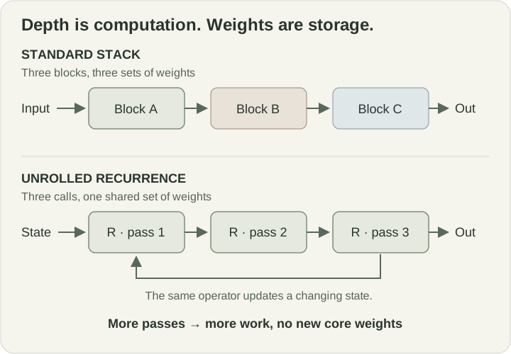
Figure 1. The repeated boxes in the lower row are calls to the same parameters. They are separate operations in the computation graph, so they still consume time and produce different activations.
can vary at test time. The architecture does not hard-code a maximum number of passes. Training over a distribution of depths can make additional passes useful, but weight sharing alone does not guarantee improvement or stable extrapolation.
The state is latent and shared across positions. Each pass updates the full sequence representation. Attention exchanges information across positions subject to its mask: an encoder may attend bidirectionally; a causal decoder such as Huginn only attends to the available prefix. Recurrence is across depth, while positions within a pass can be processed in parallel during prefill or training. Autoregressive generation still produces successive output tokens sequentially.
What stays fixed, and what grows?
Let be the core’s parameter count, the embedding/prelude/coda parameters, and the work of one core pass. The following is simple accounting, rather than a claim about measured throughput:
The first line does not depend on ; the next two do. More loops reduce the need for distinct weights at a given effective depth, while still paying for the repeated operations. Actual latency also depends on memory traffic, kernels, batching, and the cache policy.
Comparing like with likeSaunshi et al. write for a -layer model looped times. Their iso-parameter baseline is : the same core parameter budget, fewer operations. Their iso-FLOP baseline is : comparable effective depth and compute, more distinct weights. Keep the common embedding and output layers in mind when interpreting parameter ratios. Reasoning with Latent Thoughts, §2
Anatomy of one loop pass
What exactly happens to information during one recurrence? Using the Huginn design [6] as the reference (it is the most carefully documented), a token’s journey is:
1. Prelude. Tokens are embedded (scaled by ) and passed through a small stack of ordinary, non-shared layers P. Output: an initial working representation . The prelude runs once.
2. State initialization. The recurrent state is not the prelude output - it is sampled from a truncated normal distribution (variance 2/5 in Huginn). The state starts as structured noise; the loop’s job is to shape it.
3. The loop body. Each iteration: concatenate with the prelude output along the hidden dimension, and map each -vector back down to through a learned adapter matrix . (Addition instead of concatenation works equally well at small scale; concatenation won at 3.5B.) Then run the shared transformer layers, and rescale the output with an RMSNorm. So per iteration, every position: reads the current state of all positions via attention, mixes in a fresh copy of the input via the adapter, and writes its updated state.
4. Coda. After iterations, a few more non-shared layers plus the unembedding (tied to the input embedding) map the final state to logits.
Written as tensor operations, that path is:
The semicolon denotes concatenation along the hidden dimension, and is the shared stack inside the core. includes the final vocabulary projection and normalization to probabilities. The input representation is re-injected on every pass. Huginn, §3
Shared weights do not imply identical KV activations. Different passes generally have different hidden states, hence different keys and values. Huginn separately experiments with a cyclic cache: iteration writes to slot for a budget of recurrent steps. Its four-step cache scores 5.86 on MT-Bench with no statistically significant drop in that experiment; this is empirical cache compression, not an architectural guarantee. Huginn, §6.2
What truncated backprop actually optimizes
The sampled-depth objective averages over both training examples and the number of recurrent passes:
Full backpropagation differentiates through every pass. Truncation computes the early passes without retaining their gradient graph, detaches that state, and differentiates through only the final passes. Huginn uses . Huginn, §3.3
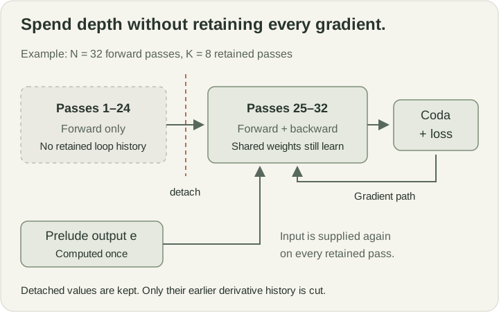
Figure 2. Forward computation still runs through all passes. Only the last passes retain the recurrent gradient history. A detached state keeps its numerical value and cuts the derivative through its earlier computation.
For a concrete derivation, define the state Jacobian and the direct parameter derivative . Ignoring shell terms and assuming is independent of , full differentiation obeys
Truncation replaces the true with zero at the detach boundary. The late terms still train the shared weights, but early contributions propagated through chains of Jacobians are omitted. This is a biased approximation to the full gradient; it is not equivalent to training a shallower forward model. Because is used again after detachment, the prelude can still receive gradients through those retained uses.
This distinction explains the memory benefit: recurrent activation storage scales with the retained window , while forward work still scales with . Reusing parameters saves weight memory; truncating gradients saves training activation memory. They solve different accounting problems.
When should the loop stop?
A useful stopping signal is whether the prediction has changed, rather than simply counting passes. For vocabulary distributions and at the position being decoded, one possible rule is
Here avoids immediate exits and caps compute. This is an illustrative rule: its threshold, minimum depth, and any requirement for several consecutive stable predictions must be evaluated for the model and task. Huginn experiments with successive-output KL divergence for early exits. Huginn, §6.1
Stability is not correctness. A wrong answer may be stable, while a useful hidden trajectory may keep moving even when its decoded answer is stable. Measuring exit accuracy against a fixed-depth baseline is therefore part of evaluating the stopping policy. Reading the coda to inspect predictions also costs compute.
The lineage, with details
2018 - Universal Transformer. Dehghani et al. [1] start from an observation that still motivates the field: vanilla transformers fail to generalize on simple algorithmic tasks - copying strings, executing short programs - once inputs exceed training lengths, while recurrent models handle those trivially. Their fix is to apply one shared encoder/decoder block repeatedly over the whole sequence at once, with two additions: a per-step time embedding added to the position encoding so the shared block knows which iteration it is on, and dynamic halting (ACT, from Graves 2016 [17]): each position maintains a halting probability that accumulates over iterations; when the cumulative mass passes , that position stops updating and its state is copied forward unchanged. So even in 2018 the loop count was per-position and data-dependent. Results: SOTA on bAbI question answering at the time, a new SOTA on LAMBADA language modeling, +0.9 BLEU over the base transformer on WMT14 En-De, and a proof that under mild assumptions the UT is Turing-complete while the fixed-depth transformer is not. The paper framed the UT as “a parallel-in-time self-attentive recurrent sequence model” - every looped transformer paper since is a variation on this sentence.
2019 - ALBERT. Lan et al. [2] tie all layer weights in a BERT-scale model and lose remarkably little accuracy while cutting parameters by roughly 10x. Not a reasoning paper - a parameter-efficiency paper - but it established the load-bearing empirical fact the whole field leans on: depth-wise weight sharing is nearly free in quality. If tying weights barely hurts at fixed depth, the door is open to tie weights and vary depth.
2023 - Looped transformers as programmable computers. Giannou et al. [4] ask the expressiveness question and answer it constructively. With hand-set weights, a constant number of encoder layers in a loop can implement: a scratchpad with read/write via attention-based copying, a program counter, conditional branching (if cond then goto), and function calls. Assembled, these emulate a one-instruction-set computer (SUBLEQ is Turing-complete), and the input sequence acts as a punchcard holding both program and data. Their headline artifact: a 13-layer looped transformer that, instructed entirely by its input, runs a calculator, a small linear algebra library, and - the foreshadowing - an in-context learning algorithm that internally performs backpropagation with SGD. Existence result, hand-programmed, not learned: it proves the architecture can express general computation at constant depth, not that gradient descent will find it. That gap is what the next three years of papers attacked.
2024 - Length generalization. Fan et al. [5] pick up the UT’s original failure case with modern tools. They study tasks whose solutions are repeated applications of one RASP-L operation (parity, copy with repeats, binary addition/sum/multiplication, unique-set), and train looped transformers with a randomized number of loop steps per training batch - the single most copied trick in the field since. Two results matter: looped models length-generalize far beyond the training lengths where fixed-depth transformers collapse, and at inference a simple maximum-confidence stopping criterion (halt when the output distribution stops changing) recovers the right number of loops per input. Learn the local update; let the runtime supply the iterations.
Worked example: ripple-carry addition
Addition makes the computation concrete. First, check : the units create a carry, the tens absorb it, and the hundreds create the final leading digit. There is no carry from the tens into the hundreds because . This example does not require a carry to ripple through the full number.
For a true carry chain, use . Give each decimal column its own state and let one synchronous update read the carry from the column immediately to its right. This is a hand-specified algorithm illustrating recurrence, not a claim that a trained model necessarily uses this exact circuit.
Define one local update
Index columns from the units upward: . Let be the fixed input digits, and let be the carry entering column at pass . Initialize every carry to zero and keep . Then
All columns update at once using the previous pass’s carries. The raw operand digits remain fixed, so a carry is never accidentally added twice to an already-updated digit.
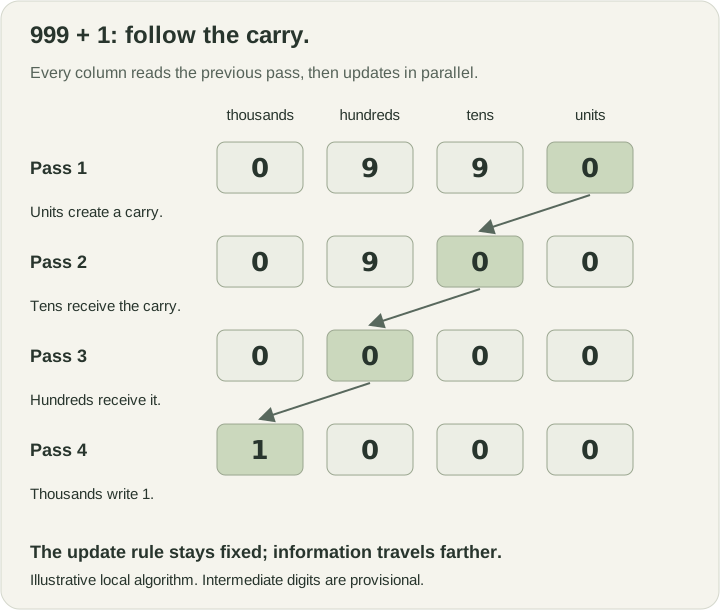
Figure 3. Provisional output digits need not form the correct sum until the carries settle. The fourth pass writes the leading 1 into a padded thousands column.
| Pass | Carries entering thousands / hundreds / tens / units | Provisional digits |
|---|---|---|
| 1 | ||
| 2 | ||
| 3 | ||
| 4 |
Under this update rule, produces provisional after the first pass and the correct after the second. In contrast, a run of nines propagates new information one column per pass. This is a statement about this local algorithm; addition also admits parallel carry algorithms, and the architecture alone does not impose this schedule.
What the example teaches
The reusable operation can be small. The block only needs to implement a digit sum, a remainder, and a neighboring carry read. The parameter budget describes the update rule; the iteration count determines how far information can travel under that rule. Saunshi et al.’s learned one-layer model looped 12 times nearly matches their 12-layer addition baseline. Reasoning with Latent Thoughts, Table 1
The necessary depth depends on the input and representation. Longer carry chains need more passes for this construction, but merely increasing a learned model’s depth does not prove length generalization. The model must learn an update that remains useful outside its training distribution. Fan et al. investigate this empirically with randomized recurrence depths. Looped Transformers for Length Generalization
The general pattern is iterative refinement. Graph message passing, relaxation methods, and gradient descent also repeatedly apply an update to a working state. Giannou et al.’s hand-programmed transformer constructions make the expressiveness connection precise; they do not guarantee that ordinary training discovers those constructions. Looped Transformers as Programmable Computers
Inside Huginn: the recurrent-depth recipe
Geiping et al. [6] (University of Maryland / ELLIS; model code-named Huginn) is the paper that answered “does any of this survive real pretraining scale?” The answer came with receipts, including the failed runs. This section is the recipe in full.
The model
Decoder-only transformer with the prelude / loop / coda split described above. Its shape is : two prelude layers, four shared recurrent layers, and two coda layers.
| Quantity | Huginn configuration |
|---|---|
| Hidden width | |
| Attention | 55 heads, 96 dimensions per head |
| MLP inner width | 17,920 |
| RMSNorm epsilon | |
| Prelude + head | About 1.5B parameters |
| Shared recurrent block | About 1.5B parameters |
| Tied embedding | About 0.5B parameters |
| Total | About 3.5B parameters |
| Nominal training recurrence |
At 32 recurrent passes, the effective depth is
Model: tomg-group-umd/huginn-0125. Training code: seal-rg/recurrent-pretraining.
The training recipe
Sampled loop counts. Each micro-batch draws its recurrence depth from a log-normal Poisson mixture. Expressing the normal distribution with an explicit variance parameter,
The shift by one guarantees at least one pass. With this parameterization ; the paper nevertheless uses as its nominal recurrence setting and to set the initialization scale. Typical draws are shallower, with a long right tail that exposes the model to deeper computation. A single sampled is synchronized across workers for each micro-batch to avoid workers waiting on different unroll depths.
Truncated backprop. Only the final iterations retain recurrent gradients, as derived above. This bounds recurrent activation memory and backward work independently of the sampled . Re-injecting lets the prelude receive gradients through the retained iterations.
Initialization. The model uses truncated-normal weight initialization, with small output projections to stabilize a deep residual computation:
The initial recurrent state is sampled afresh with variance . Embeddings are scaled by .
The two failed runs. The paper documents what happens if you skip this: “Bad Run 1” used parameter-free RMSNorms, no embedding scale, a parameter-free additive adapter (), and peak LR . The run stalled, and the stall mechanism is diagnostic gold: the correlation of hidden states across the token dimension goes to 1.0 - the model’s representation collapses, predicting the same hidden state for every token. A second failed run collapsed the recurrence itself (the loop degenerated to near-identity). The sandwich of learned norms, scaled embeddings, concatenation adapter, and small out-projection init is not decoration; it is what makes the loop a loop.
The run
Trained on the Frontier supercomputer (Oak Ridge; 9408 nodes of AMD MI250X) in 21 segments of up to 12 hours each, mostly in December 2024, on up to 4096 GPUs at 41-51% achievable-FLOP utilization, ~1-1.2M tokens/second, global batch 16M tokens, bf16, data-parallel only (weight sharing keeps the model small enough to skip tensor parallelism). AdamW with , learning rate , constant schedule with 4096-step warmup, gradient clip 1.0. Because the LR was constant, extra segments were bolted on whenever allocation appeared, to a final 795B tokens. A feedforward twin (same everything, one pass through the core block) was trained on 180B tokens as the control.
The results, with numbers
Zero-shot lm-eval-harness at 800B tokens, as a function of test-time recurrence r (Table 1 of the paper):
Table 1. Huginn-3.5B zero-shot accuracy versus test-time recurrence. Scores are percentages; training-token budgets are shown in each model label.
| Benchmark | ||||
|---|---|---|---|---|
| ARC-E | 49.07 | 65.11 | 69.49 | 69.91 |
| ARC-C | 27.99 | 35.15 | 37.71 | 38.23 |
| HellaSwag | 43.46 | 58.54 | 64.67 | 65.21 |
| MMLU | 23.39 | 25.29 | 31.25 | 31.38 |
| OBQA | 28.20 | 35.40 | 37.60 | 38.80 |
| PiQA | 64.96 | 73.45 | 75.79 | 76.22 |
| SciQ | 80.00 | 92.10 | 93.90 | 93.50 |
| WinoGrande | 55.24 | 55.64 | 57.77 | 59.43 |
Reference models from the same reported table. These differ in size and training budget, so they are context rather than controlled ablations.
| Benchmark | Pythia 2.8B / 0.3T | Amber 7B / 1.2T | OLMo-2 7B / 4T |
|---|---|---|---|
| ARC-E | 58.00 | 65.70 | 82.79 |
| ARC-C | 32.51 | 37.20 | 57.42 |
| HellaSwag | 59.17 | 72.54 | 80.50 |
| MMLU | 25.05 | 26.77 | 60.56 |
| OBQA | 35.40 | 41.00 | 46.20 |
| PiQA | 73.29 | 78.73 | 81.18 |
| SciQ | 83.60 | 88.50 | 96.40 |
| WinoGrande | 57.85 | 63.22 | 74.74 |
Read it honestly. Going from to buys +20.8 points on ARC-E and +9.0 on MMLU at zero training cost. But also note the last row: OLMo-2 7B (4T tokens) beats it everywhere, and Huginn’s MMLU at 31.4 is weak in absolute terms. The paper’s claim is about the direction - a knob that exists and works - not about SOTA. Saturation is task-dependent: HellaSwag is close to its score by , GSM8K keeps improving to . On ARC-C the saturation point shifts later with more few-shot examples: more context in, more loops used. The model spends compute in proportion to what it’s given.
Three findings that didn’t fit in the table:
The gains live in the loop, not the shell. Evaluated at , the model flatlines between the 180B and 800B checkpoints - all improvement from the extra 600B tokens is encoded in the iterated block, not the prelude or coda. Against its feedforward twin at 180B, the recurrent model is already ahead everywhere, and on GSM8K it is 5x better. The authors’ “equivalent to a 50B-parameter compute load” headline comes from this direction of comparison.
Free inference-time features. Because is a runtime choice, the model gets three things zero-shot that standard transformers need whole research programs for: per-token adaptive compute (exit when the state stops changing - on MMLU the model ponders ~3.5 steps longer on moral-scenarios questions than on high-school math, with no training for this); self-speculative decoding (draft tokens with few iterations, verify with more - no separate draft model); and KV-cache sharing (cyclic cache budget of 4 steps costs nothing on MT-Bench: 5.86).
The latent space is doing recognizable geometry. Tracking token trajectories : most tokens converge to fixed points, but key tokens in hard questions trace orbits (loops in latent space, observed on arithmetic), and some tokens are sliders - steady drifts in one direction, which can implement iteration counting. These behaviors were never in the training objective; they emerged with scale. And the dynamics are path-independent: re-initialize and the same orbits and fixed points reappear.
Latent thoughts: the reasoning/memorization split
Saunshi, Dikkala, Li, Kumar, Reddi (Google DeepMind; ICLR 2025) [3] is the cleanest argument for why loops should help reasoning specifically, built in four claims.
Claim 1: reasoning needs depth, not parameters
On three procedurally generated tasks - n-ary addition, p-hop induction (a recursive backtracking version of induction heads), and i-GSM (symbolic math word problems with 7B+ unique solution templates) - a looped model nearly matches the iso-FLOP 12-layer baseline and crushes the iso-param k-layer model, on input difficulty far beyond the training mix. The extreme data point: 1 layer looped 12 times solves addition with 1/12th the parameters. The theory section backs this: problems solvable by iterative algorithms with short descriptions are solvable by looped models at nearly optimal depth - the loop count tracks the problem’s iteration complexity, not its size.
Claim 2: in language modeling, loops trade perplexity for reasoning
This is the paper’s most interesting empirical move. They pretrain 24-layer, 1B-parameter GPT-2-style models on 250B tokens of the Pile, then compare the looped against both baselines on 25 downstream tasks grouped into memorization-flavored (closed-book QA) and reasoning-flavored (open-book QA, math word problems, reasoning primitives) buckets. The numbers for :
Table 2. Pile-pretrained models: perplexity and downstream task scores. Lower perplexity is better; higher task scores are better.
| Metric | Baseline | Shallow | Loop | Middle loop |
|---|---|---|---|---|
| Architecture | ||||
| Params/FLOPs | 24x/24x | 12x/12x | 12x/24x | 12x/24x |
| PPL ↓ | 7.40 | 8.16 | 7.90 | 7.81 |
| Closed-book QA | 11.2 | 8.2 | 9.3 | 11.0 |
| Open-book QA | 33.9 | 26.9 | 30.8 | 32.3 |
| Math word | 29.3 | 26.7 | 34.3 | 28.3 |
| All-task avg | 26.0 | 21.8 | 26.5 | 25.0 |
| Reasoning primitives | 47.5 | 35.7 | 51.2 | 56.5 |
The dichotomy, in one table. The looped model has worse perplexity than the iso-FLOP baseline (7.90 vs 7.40) - memorization capacity tracks parameters, and it has half of them. But it closes 131% of the gap on reasoning primitives (i.e., beats the 24-layer baseline outright with half the parameters), and the middle-loop variant - unique layers at the ends, loop in the center - does even better at 56.5, nearly matching the baseline on closed-book QA. Their ”% Gap” metric shows the pattern across all k: loops close little of the memorization gap (34-37%) and most or all of the reasoning gap (56-282%). Perplexity and downstream reasoning decouple. Facts live in parameters; multi-step inference lives in depth.
Claim 3: loops generate latent thoughts, and can simulate CoT
Their conceptual framing: a CoT model is a loop that emits one thought-token per iteration; a looped model emits a full latent state per iteration - strictly more bandwidth. Formally, they prove a looped model with a scratchpad can simulate steps of CoT with loops. Empirically, downstream accuracy scales with the log of effective depth for both looped and non-looped models, structurally the same law as CoT scaling with generated tokens. Looping is CoT in continuous space, with the same scaling shape and a much wider channel.
Claim 4: you can get some of the benefit without looping
Inspired by the inductive bias, they add a regularizer that pulls successive layers of a non-looped model toward functional similarity. It inherits part of the reasoning benefit with no perplexity cost - evidence that “layers that can survive being iterated” is itself a useful training signal, not just an architecture.
HRM: hierarchy as a stability trick
The Hierarchical Reasoning Model [8] (Wang et al., Sapient Intelligence) attacks a different failure of loops than efficiency: training stability at extreme effective depth. A weight-tied loop is a dynamical system, and a naive one either converges instantly (later iterations become inert) or explodes. HRM’s answer, borrowed from multi-timescale processing in the brain, is two coupled recurrent modules: a low-level module that updates fast, and a high-level module that updates once per cycle of low-level steps - and when updates, ‘s state is reset to start a fresh phase. They call this hierarchical convergence: the fast module is repeatedly driven to a local equilibrium, the slow module moves only on equilibria, and the system avoids both premature convergence and blow-up. Over cycles of steps with 4-layer modules and up to deep-supervision segments, the effective depth reaches layers - an absurd depth that trains stably at 27M parameters.
No backprop through time. HRM trains with a one-step gradient approximation, justified via deep equilibrium models: if converges to a fixed point given , the implicit function theorem gives the gradient of the fixed point without unrolling. In practice: backprop only through the last and step, and between supervision segments the state is detached from the graph. Memory stays in depth instead of BPTT’s . The TRM paper later showed the fixed-point assumption is barely true at the moment it’s invoked - more on that below.
Deep supervision and halting. Training runs up to 16 segments per example: each segment forward-passes from the previous segment’s (detached) state, computes a loss, updates. A Q-learning head on the final predicts Q-values for “halt” vs “continue” - Adaptive Computation Time - so easy examples stop early (under 2 segments on average on Sudoku-Extreme, vs 16 max), while all 16 are used at test time. Architectural odds and ends that matter at this scale: Post-Norm blocks, RoPE, SwiGLU, stablemax instead of softmax for small-data generalization, Adam-atan2 optimizer, fixed random initial state.
The results that went viral: trained from scratch on ~1000 examples per task, no pretraining, no CoT: near-perfect Sudoku-Extreme and optimal pathfinding on 30x30 mazes - tasks where o3-style CoT models score 0% - and 40.3% on ARC-AGI-1 with a 900-token context, above o3-mini-high (34.5%) and Claude 3.7 8K (21.2%). 27 million parameters.
TRM: how much of HRM was actually necessary
Alexia Jolicoeur-Martineau’s Tiny Recursive Model [9] (Samsung SAIL Montréal) is a controlled demolition of HRM’s machinery, and the most instructive paper in the whole area for how to read this literature. Her moves, each ablated on Sudoku-Extreme (1K train, 423K test):
Drop the fixed-point theory entirely
HRM’s one-step gradient is justified by the IFT at a fixed point - but TRM checks the residuals and finds is nowhere near converged when the theorem is invoked. So TRM simply backprops fully through one complete recursion process (n updates of the latent plus 1 answer update) and keeps the BPTT-free segments on top. No theorem needed, and generalization jumps: 56.5% → 87.4% on Sudoku-Extreme.
Reinterpret the two features
The biological “hierarchy” story dissolves under inspection: is just the current answer (apply the output head and argmax and you read it off), and is a latent reasoning scratchpad. So TRM renames them y and z: the network updates the reasoning z given (question x, current answer y, current z), then updates the answer y given (y, z). Why exactly two features? Because z plays the role a chain-of-thought would - drop it and the model forgets how it got its answer; drop y and the model is forced to store its answer inside its reasoning channel. Splitting z into more features hurts (77.6%), collapsing to one hurts (71.9%). Two is the natural number, no brain required.
One network, not two
The low-level update sees x () and the high-level update doesn’t () - the task is fully specified by whether x is in the input. So a single network can do both jobs: 82.4% → 87.4%, at half the parameters.
Less is more, literally
Adding layers hurt; removing them helped. With only ~1000 training examples, a 4-layer net overfits; a 2-layer net with proportionally more recursions (same effective depth) generalizes best: 79.5% → 87.4%, half the parameters again. Echoes of fixed-point diffusion models, where 2 layers were also optimal.
Attention is optional on small grids
When context length , where is the hidden width, a token-mixing MLP (à la MLP-Mixer) is cheaper than attention’s projections and generalizes better: +10 points on Sudoku. It loses on the 30x30 tasks, so TRM keeps attention there - architecture per task, not one architecture for everything.
Cheap halting and stability
HRM’s Q-learning ACT needs a second forward pass; TRM replaces it with a plain binary-cross-entropy “is the answer correct yet” head (86.1% → 87.4%, one pass). And an EMA over weights stops the overfit-then-diverge pattern on tiny data (79.9% → 87.4%).
The resulting model. One 2-layer, 5M-parameter network, answer updates of latent recursions each (effective depth 42 per supervision step, up to 16 steps): 87.4% Sudoku-Extreme (HRM: 55.0%), 85.3% Maze-Hard (74.5%), and with the 7M attention variant, 44.6% ARC-AGI-1 and 7.8% ARC-AGI-2 - vs HRM’s 40.3% / 5.0% at 4x the parameters, and vs Gemini 2.5 Pro’s 37.0% / 4.9% and o3-mini’s 34.5% / 3.0%. Only Grok-4-thinking (66.7% / 16.0%, ~1.7T parameters) sits clearly above among LLMs.
Table 3. Sudoku-Extreme accuracy at approximately comparable effective depths. The two models do not have exactly equal depths.
| Effective depth / step (HRM / TRM) | HRM (4 layers) | TRM (2 layers) |
|---|---|---|
| ~9 / 7 | 46.4% | 63.2% |
| 24 / 20 | 55.0% | 81.9% |
| 48 / 42 | 61.6% | 87.4% |
| 80 / 72 | 59.5% | 84.2% |
| 168 / 156 | 57.5% | OOM |
Depth helps until it doesn’t. Both models improve with effective depth up to a sweet spot, then degrade (HRM) or run out of memory (TRM backprops through the full recursion, so deep unrolls OOM). Depth is a dial with an optimum, not a monotonic good - the same saturation shape as Huginn’s test-time curves.
What people are saying
The reaction to this wave has been unusually two-sided, and the critical literature is as informative as the papers.
The ARC Prize Foundation’s audit [13] is the centerpiece. HRM went viral in June 2025 (4M+ views on X threads, 475K+ on YouTube). The Foundation scored it on the hidden semi-private sets and ran ablations. Findings: it approximately reproduces (32% ARC-AGI-1, 2% ARC-AGI-2 on the hidden sets, vs 40.3%/5.0% public) - impressive for the size, not state of the art, and “not material progress on ARC-AGI-2.” More importantly, where the performance comes from: the hierarchical architecture itself had minimal impact over a same-size plain transformer; the “outer loop” of deep-supervision refinement drove the gains (deep supervision roughly doubled accuracy, 19% → 39%; hierarchical recursion added only 35.7% → 39.0%); cross-task transfer was limited - much of the score is memorizing solutions to the specific evaluation tasks, which ARC-AGI supplies at eval time; and task augmentation was critical (though ~300 augmentations sufficed, not the 1000 used). Their conclusion: the approach is “fundamentally similar” to an existing augment-and-refine pipeline, and the brain-inspired framing oversold the mechanism.
TRM’s author says the quiet part too [9,14]: “the question of why recursion helps so much compared to using a larger and deeper network remains to be explained; we suspect it has to do with overfitting, but we have no theory.” And these models are supervised, deterministic input-output machines, not generative models - nothing here writes a poem, and extending the trick to generative tasks is explicitly future work.
Is there a latent chain-of-thought? A follow-up probing study of Huginn [15] (Logit Lens and a purpose-built “Coda Lens” on arithmetic) found limited evidence of interpretable latent CoT: the intermediate loop states do not decode into clean intermediate calculations the way token-level CoT does. The loop is doing something structured (orbits, sliders, path-independent dynamics per the original paper), but it is not a readable reasoning trace. For alignment-minded readers this is the sharpest concern in the whole area: latent reasoning’s advantage - no tokens - is also its audit problem.
The 2026 mechanistics wave is trying to close exactly that gap. The convergence-selection paper [11] argues that standard representational-similarity metrics are “tail instruments”: they provably saturate at the fixed points loops converge to, while the algorithm lives in the head of the trajectory. Their proposed head instrument - convergence-time scaling , the first loop at which position i’s decoded output stabilizes - is validated causally by activation patching, predicts which training seeds generalize (tail metrics don’t), and reproduces on the public easy-to-hard benchmark with 4x exact-match length extrapolation. DeepLoop [10] attacks the stability side: a DeepNorm-style scaling rule for Post-LN looped blocks (, ), derived from a depth-untied bound, with GPT-2-small/medium ablations showing the correction matters precisely when loop count exceeds one. And the ARC Prize analysis plus TRM together reset expectations for the tiny-reasoner claims: recursion works, but via supervision steps, augmentation, and refinement more than via any single architectural idea.
The meta
Why is this resurging now, when the Universal Transformer was 2018? Three forces converged. First, the complexity ceiling got formalized: fixed-depth transformers sit in -like classes and provably can’t do polynomial-time sequential computation end-to-end; CoT escaped that ceiling by spending tokens, and loops escape it by spending depth - after o1 made test-time compute the frontier, every lab needed a position on all the ways to spend it. Second, the economics: FLOPs are cheap and getting cheaper, while parameters are what you pay to store, ship, and serve - a loop trades exactly the cheap resource for the expensive one, and recurrent KV-cache sharing can reduce the activation-memory cost. Third, the tooling caught up: randomized-depth training, truncated backprop, and modern init/norm schemes (each rediscovered the hard way, cf. Huginn’s collapsed runs) made loops trainable at scale for the first time.
Who is betting. The affiliations are the tell: Google DeepMind on both the theory (Saunshi et al.) and the adaptive-efficiency side (MoR, with KAIST and Google Cloud); UMD/ELLIS with the open 3.5B proof-of-concept; Samsung SAIL Montréal on tiny recursive reasoners; Sapient Intelligence’s whole company bet on HRM; ByteDance Seed appearing in the recurrent-depth citation graph by 2026 [11]; Meta FAIR adjacent via continuous-thought (Coconut [16]), which loops at the token level by feeding hidden states back as embeddings - the same idea one axis over. This is no longer a niche; it is a named contender for the post-CoT scaling direction, with frontier labs holding positions.
The honest synthesis. Loops buy: test-time compute without tokens, parameter efficiency, depth-on-demand, and strong wins on iterative/verifiable domains. They cost: worse memorization per FLOP (Saunshi’s perplexity gap, Huginn’s 31.4 MMLU), a saturation ceiling set by training depth, harder serving (variable per-token depth vs. batch-parallel hardware; MoR’s expert-choice routing is the current best answer [7]), opaque internal computation, and - per the ARC audit - a tendency for headline claims to decompose into more mundane mechanisms on inspection. The most defensible 2026 position is that recurrence over depth is a real, load-bearing third axis of scale that composes with the other two - not a replacement for parameters, and not (yet) a replacement for chain-of-thought.
Open questions
1. Why does recursion beat a bigger, deeper network at all? TRM’s author names it directly: suspected overfitting control, no theory. Saunshi’s regularizer result hints the inductive bias itself is the active ingredient. Nobody has the account.
2. Saturation. Every test-time curve in this literature bends over - Huginn’s by task, TRM/HRM by depth, with OOM or degradation past the sweet spot. Training-depth distributions, loop-aware normalization (DeepLoop), and curriculum over depth are all being tried; nobody has a curve that rivals token-scaling all the way up.
3. Reading the loop. Latent CoT probing found little that is human-legible; convergence-time instruments are the first mechanistic handle. Faithful auditing of 32 iterations of continuous thought is the alignment problem for this whole direction.
4. Generative tiny reasoners. HRM/TRM are supervised one-answer machines. Making recursive refinement generative (multiple valid answers, open-ended outputs) without losing the small-data magic is unsolved.
5. Systems. Per-token variable depth fights batch-parallel serving. MoR’s expert-choice routing and continuous depth-wise batching are the start; a serving stack that treats loop count as a first-class scheduling dimension doesn’t exist yet.
6. Composition. Depth loops, token loops (CoT/Coconut), tool use, and retrieval are four independent axes of test-time compute. Almost nothing is known about their interactions - multiply, substitute, or interfere. The interesting 2027 paper lives there.
References
- Dehghani, Gouws, Vinyals, Uszkoreit, Kaiser. Universal Transformers. 2018. arXiv:1807.03819
- Lan et al. ALBERT: A Lite BERT for Self-supervised Learning of Language Representations. 2019. arXiv:1909.11942
- Saunshi, Dikkala, Li, Kumar, Reddi. Reasoning with Latent Thoughts: On the Power of Looped Transformers. ICLR 2025. arXiv:2502.17416
- Giannou, Rajput, Sohn, Lee, Lee, Papailiopoulos. Looped Transformers as Programmable Computers. ICML 2023. arXiv:2301.13196
- Fan, Lou, et al. Looped Transformers for Length Generalization. 2024. arXiv:2409.15647
- Geiping, McLeish, Jain, et al. Scaling up Test-Time Compute with Latent Reasoning: A Recurrent Depth Approach. 2025. arXiv:2502.05171
- Bae et al. Mixture-of-Recursions: Learning Dynamic Recursive Depths for Adaptive Token-Level Computation. NeurIPS 2025. arXiv:2507.10524
- Wang et al. (Sapient Intelligence). Hierarchical Reasoning Model. 2025. arXiv:2506.21734
- Jolicoeur-Martineau (Samsung SAIL Montréal). Less is More: Recursive Reasoning with Tiny Networks. 2025. arXiv:2510.04871
- DeepLoop: Depth Scaling for Looped Transformers. 2026. arXiv:2607.13491
- When Does Recurrence Become an Algorithm? Convergence Selection in Weight-Tied Looped Transformers. 2026. arXiv:2607.20594
- Goyal et al. Think Before You Speak: Training Language Models With Pause Tokens. 2023. arXiv:2310.02226
- ARC Prize Foundation. The Hidden Drivers of HRM’s Performance on ARC-AGI. Aug 2025. arcprize.org/blog/hrm-analysis
- Jolicoeur-Martineau. Tiny Recursion Models (author’s blog post). Sep 2025. alexiajm.github.io
- Latent Chain-of-Thought? Decoding the Depth-Recurrent Transformer. 2025. arXiv:2507.02199
- Hao et al. (Meta FAIR). Training Large Language Models to Reason in a Continuous Latent Space (Coconut). 2024. arXiv:2412.06769
- Graves. Adaptive Computation Time for Recurrent Neural Networks. 2016. arXiv:1603.08983
- Bai, Kolter, Koltun. Deep Equilibrium Models. NeurIPS 2019. arXiv:1909.01377
Eternal Horizons · a #evergreen note - permanent, constantly growing. Companion piece to Transformers from first principles. Format modeled on the Transformer Circuits article style.